안녕하세요. 이번에는 Rshiny에서 highcharts 패키지로 그래프를 그려보겠습니다.
highcharter R 패키지는 R 개체를 플롯하는 바로 가기 기능을 포함하는 'Highcharts' 라이브러리용 래퍼입니다. 'Highcharts'는 http://www.highcharts.com/ 간단한 구성 구문으로 다양한 차트 유형을 제공하는 차트 라이브러리입니다.
[목차]
1. Rshiny 서버 구축하고 highcharts 단일 그래프 그리기
2. Rshiny 서버에서 highcharts로 여러 그래프 배열
1. shiny 서버 구축하고 highcharts 단일 그래프 그리기
app.r
rm(list=ls())
gc()
sessionInfo()
Sys.setenv(R_HOME="C:/Program Files/R/R-4.1.1")
library(here)
...

ipconfig <- trimws(strsplit(grep("IPv4",system("ipconfig", intern=TRUE), value = T),":")[[1]])[2]

source("server.R", encoding = "UTF-8")
source("ui.R",  encoding = "UTF-8")
source("websocket.R",  encoding = "UTF-8")

runApp(app= shinyApp(ui = ui,server = server), host=getOption("shiny.host", ipconfig),test.mode = getOption("shiny.testmode", FALSE), port=3898)
위는 app.r 코드로 마지막줄 runApp을 구동하기 위해서 ui 객체와 server 객체를 입력해주는 코드입니다.
library(here)는 패키지 페이지에서 보듯이 기본 폴더를 기준으로 하위 폴더 인용을 쉽게 도와줍니다.
ipconfig는 현재 ip 확인을 위해서 수행한 것이며 편의상 중간을 ...으로 생략했고 주요한 내용만 남겼습니다.
ui.r
body <- dashboardBody(
   ## 3.0. CSS styles in header ----------------------------
   tags$head(

...

),


      ## 3.1 stock - stock info  -----------------------------------------------------
      tabItem( tabName = 'stock_info',
               tags$div( id = 'div_stock_info_page' ,
                         fluidRow( h1( "stock Information." ),
                                   uiOutput("ui_select_stock_info"),
                                   dateRangeInput('dateRange',
                                                  label = 'Date range input: yyyy-mm-dd',
                                                  start = get.my.stockdate(dateCount=5)[3], end = get.my.stockdate(dateCount=5)[1]
                                   ),
                                   div( id = 'div_btn_stock_chart',
                                        tags$style(type="text/css", "#btn_stock_chart {background-color:DodgerBlue;color: black}"),
                                        actionButton("btn_stock_chart",
                                                     paste0('Search'),
                                                     icon = icon('search', class = "small_icon_test"),
                                                     style='padding-top:3px; padding-bottom:3px;padding-left:5px;padding-right:5px;font-size:120% '
                                        )
                                   ),
                                   highchartOutput("plot_candle_stock")
                         )
               )
      ),

...

)
ui 코드입니다.
body 로 입력되는 dashboardBody 는 shinydashboard 패키지에 존재하는 객체입니다. tabItem 또한 해당 패키지에 포함되어 있습니다. 여기서 눈여겨 볼 것은
fluidRow()
highchartOutput()
입니다.
fluidRow() 는 그래프 배열을 조절하기 위해 필수적인 함수입니다. 뒤에서 설명드리겠습니다.
한편 highchartOutput은 server 쪽에서 highchart를 이용해 그린 주식 그래프 plot_candle_stock 를 담는 것을 의미합니다.
server.r
server <- function(input, output, session){

...

...

...

  observeEvent(input$btn_stock_chart,{
    output$plot_candle_stock <- renderHighchart({
      {
        one_code<-sprintf("%06d",as.numeric(company_info[company_info$corp_name==input$select_stock_info,]$stock_code))
        fromDate<-gsub('-','',min(as.character(input$dateRange)))
        toDate<-gsub('-','',max(as.character(input$dateRange)))
        if(abs(diff(input$dateRange))>30){
          showNotification("Over 30 days.",type="error")
          return(NULL)
        }

        query<-""
        if(one_code!="")
          query<-paste0(query,'"CODE" : "',one_code,'"    ' )
        if(fromDate!="")
          query<-paste0(query,ifelse(query!="",",",""),'"TIME":{ "$gte" : "',paste0(fromDate,'090000'),'"}')
        if(toDate!="")
          query<-paste0(query,ifelse(query!="",",",""),'"TIME":{ "$lte" : "',paste0(toDate,'153000'),'"}')

        query<-paste0("{",query,"}")
        tryCatch(expr={
          content(POST(common_url, body = list(tr_type = "minSearch",code=one_code, tick=1,fix=1,size=100,
                                               nPrevNext=0,insert_flag=T, limit_count=GLOBAL_LIMIT_COUNT), encode="json", timeout(20)))
        },error=function(e){

        })
      }

      rslt_qry<-con$find(query=query)
      xx<-convert_db2Xts(db=rslt_qry,chart=T)
      xx$chart
    })

  })
이제 서버 코드입니다. 중요한 부분은 observeEvent 함수 부터입니다.
renderHighchart 는 Highchart 그래프를 의미하고 이를 plot_candle_stock output에 넣는 과정이 위 코드에 포착된 것으로 보입니다.
이를 종합하여 구동해보면 아래처럼 역동적인 삼성전자의 그래프를 확인할 수 있습니다.
highcharts는 이런 금융 데이터를 다루기에 충분히 좋습니다.

2. Rshiny 서버에서 highcharts로 여러 그래프 배열
위에서 소개한 ui.r 파일 구현의 연장선으로 여러개의 그래프를 배열하는 방법은 다음과 같습니다.
마지막 줄을 보면 fluidRow와 highchartOutput 합성된 것들이 여러개 놓여 있습니다. (highchartoutput 4개)
즉 fluidRow로 highchartOutput 여러개를 묶어서 관리했습니다.
   tabItems(
      ## 3.1 Main dashboard ----------------------------------------------------------
      tabItem( tabName = 'dashboard',
               h3(paste0("Comparison-Chart")) ,
               ## 1.2 Time serise plot ----------------------------------------
               # selectInput("sourceStock",label=c("Source Stock"),choices=c("삼성전자","LG전자"),selected = "삼성전자",
               #             multiple = TRUE,selectize = TRUE,width = NULL,size = NULL),
               dateRangeInput('dateRange',
                              label = 'Date range input: yyyy-mm-dd',
                              start = get.my.stockdate(dateCount=5)[3], end = get.my.stockdate(dateCount=5)[1]),
               div( id = 'div_btn_source_stock_chart',
                    #tags$hr(),
                    #tags$h3( "Click on the 'Show more details' button to display addtional information on free trade agreements, and imports/exports by commodities and markets." ),
                    tags$style(type="text/css", "#btn_both_stock_chart {background-color:DodgerBlue;color: black}"),
                    actionButton("btn_both_stock_chart",
                                 paste0('Search'),
                                 icon = icon('search', class = "small_icon_test"),
                                 style='padding-top:3px; padding-bottom:3px;padding-left:5px;padding-right:5px;font-size:120% '
                    )
               ),
               fluidRow(column(2,uiOutput("ui_select_source_stock_info"),uiOutput("ui_select_target_stock_info")),
               column(2,uiOutput("ui_select_source_present_info"),uiOutput("ui_select_target_present_info"))),

               fluidRow(highchartOutput("plot_candle_source_stock"),highchartOutput("plot_candle_target_stock"),
                        highchartOutput("plot_candle_source_present"),highchartOutput("plot_candle_target_present")),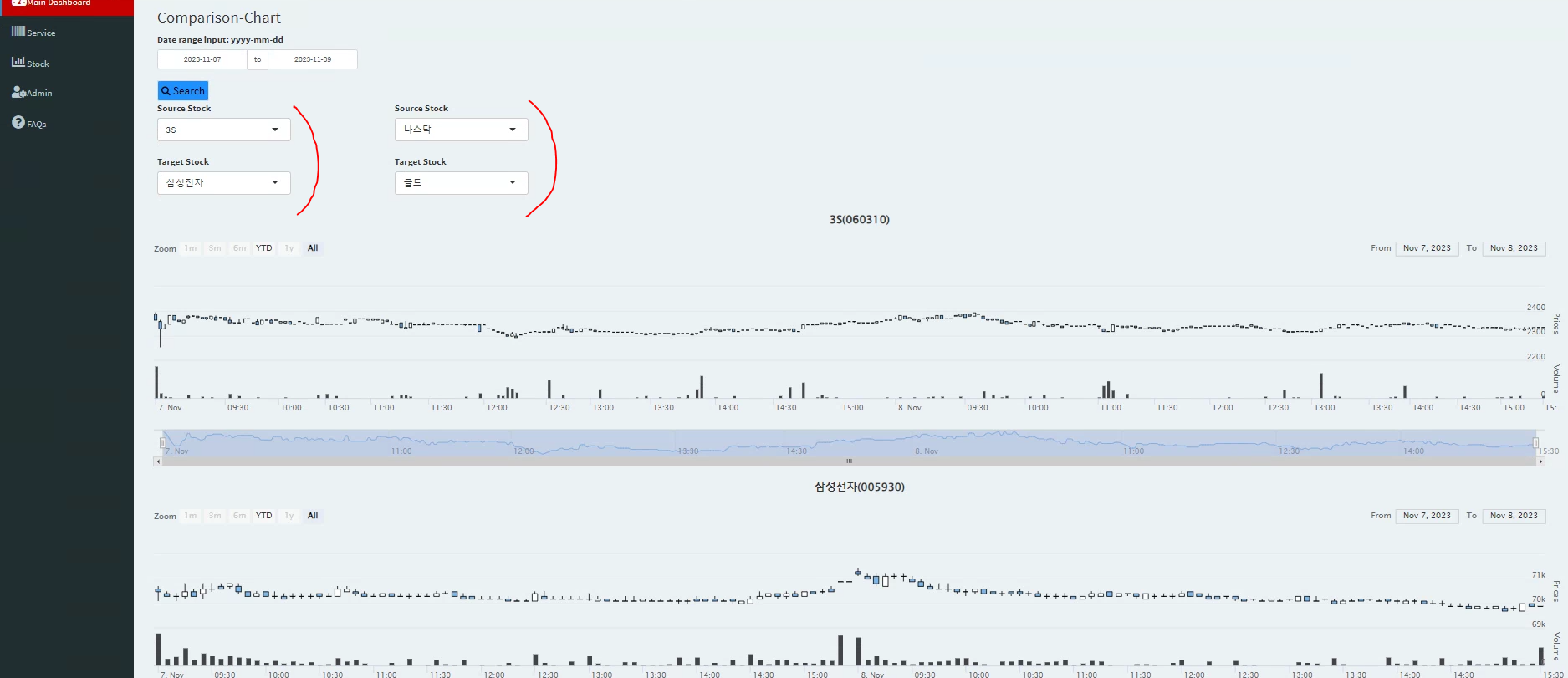
상단의 source Stock 과 Target Stock combobox는 각각 fluidrow(column(2, ... ), column(2, ...)) 이 부분에서 다뤄지고 있습니다. 참고로 바로 위 화면은 fluidrow에 highchartoutput을 4개 나열한 결과를 조회한 일부입니다. fluidRow( + highchartOutput 4개) 에서 그래프는 4개 연달아 있습니다. (2개는 화면상 더 하단에 존재) 하단으로 내리면 나스닥과 골드 선물 값을 볼 수 있습니다.
ggplot 을 이용한 예시는 다음에 찾아보겠습니다.
'정리 > 시각화' 카테고리의 다른 글
| [IDE] VSCode Python Jupyter Notebook 설정 (Markdown부터) (2) | 2023.11.20 |
|---|---|
| [R] ggplot2 서로 다른 그래프 겹치기 (1) | 2023.11.14 |
| [R] ggplot에 내가 원하는 point 그리기 (0) | 2019.10.20 |
| [R] 복수의 plot align 하기 정렬 하기 (0) | 2018.11.11 |
| [R] ggplot2 그래프 화면 분할 (0) | 2018.10.28 |


